Mean, median and mode: what each one tells you and when to use which
If a team's players scored “an average of 10 points”, did each player score 10? We explain what the mean, median and mode measure, how outliers affect them and how to choose the most suitable one for your data, with worked examples.
In this article · 9 sections
Your school basketball team scored 60 points in a match with 6 players. The next day, the school newsletter said: “Our players scored an average of 10 points in the match.” But when you look at the scoresheet, you see a very different picture: one player scored 40 points on their own, while the other five scored between 2 and 6.
So does “an average of 10” really describe this team? Mathematically, the sentence is spot on: . Yet five of the six players scored fewer than 10. In other words, summing up data with a single number can leave very different impressions, depending on which number you choose.
In this article we look at the three basic ways of summarising data: the mean, the median and the mode. With examples, we’ll see what each one measures, where it is strong and when it can mislead you. By the end, you’ll be able to look at a set of data and comfortably answer the question: “Which one should I use here?”
Three questions, three answers: what are measures of centre?
Imagine you have lots of data: a class’s test scores, a week’s daily temperatures, or the number of people living in each household on a street. Reading every value one by one is tiring. So we like to summarise the data with a single number that shows its “typical value”.
In statistics these numbers are called measures of central tendency, or simply measures of centre; in everyday maths, all three are often called types of average. You can answer the question “What is a typical value in this data?” in three different ways:
- By sharing out: if you put all the values in a bag and share them out equally, everyone’s share is the mean.
- By lining up: if you put the values in order from smallest to largest and look at the one in the very middle, that is the median.
- By looking for the crowd: if you pick the value that appears most often, that is the mode.
All three tell you something about the “centre” of the data, but each defines the centre from a different angle. So getting three different results for the same data is completely normal. What matters is knowing what each result is telling you.
The mean: sharing out and the balance point
The mean of values is their total divided by the number of values:
Here (read “x bar”) stands for the mean.
Example: Ayşe noted down how many minutes she spent reading each day for a week: 20, 35, 30, 20, 45, 20, 40.
So if Ayşe’s total reading time were shared equally across the seven days, each day would get 30 minutes.
The mean is a balance point
The mean has another lovely property. If you work out how far each value is from the mean, those differences always add up to zero. Let’s subtract 30 from each of Ayşe’s values:
That’s why you can think of the mean as the balance point of a seesaw. Picture the number line as a long plank, with each value as a marble of equal weight placed on it. If you support the plank exactly at the mean, it balances.
This picture also explains why the mean is so sensitive to extreme values. Put a single marble far out at one end of the plank, and you have to shift the support a long way towards it to keep the balance.
The mean is linked to the total
The most practical thing about the mean is that it is directly connected to the total:
Suppose you are planning a camp for 40 people and you know that each person needs an average of 2 litres of water a day. You can immediately work out that you need litres a day in total.
The median and the mode can’t give you a total like this. When the question is “How much altogether?”, the mean is indispensable.
The median: the middle of the ordered list
The median is the value in the very middle when the data is put in order from smallest to largest. Roughly speaking, half of the data lies below the median and half lies above it.
Two steps are all you need to find it:
- Put the values in order from smallest to largest.
- If there is an odd number of values, take the middle one; if there is an even number, take the mean of the two middle values.
When the number of values is odd, the median is the value in position of the ordered list. For example, with 7 values the median is the 4th; with 11 values it is the 6th.
Example (odd number of values): let’s order Ayşe’s data: 20, 20, 20, 30, 35, 40, 45. There are seven values; the 4th one, in the middle, is 30. The median is 30 minutes.
Example (even number of values): the basketball players’ points were 4, 6, 5, 3, 2, 40. In order, that’s 2, 3, 4, 5, 6, 40. There are six values; the two in the middle are 4 and 5:
The mean was 10, but the median is 4.5. We’ll discuss shortly which of the two describes this team better.
The median’s strength: robustness
The median’s most important feature is that it is robust against extreme values. What would happen if the player who scored 40 had scored 400 in an imaginary match?
- The mean would become .
- The median would still be 4.5.
That’s because the median only looks at the middle of the ordered list; it doesn’t care how large the value at the end is.
The mode: the most crowded value
The mode is the value that appears most often in the data. In Ayşe’s data, 20 appears three times, while no other value appears even twice. So the mode is 20 minutes.
It helps to know three situations involving the mode:
- One mode: in the data 3, 5, 5, 7, 8, the mode is 5.
- More than one mode: in the data 2, 2, 4, 6, 6, 9, both 2 and 6 appear twice, so there are two modes. Data like this is called bimodal.
- No mode: in the basketball data (2, 3, 4, 5, 6, 40), no value repeats. In this case we usually say “there is no mode”.
The measure for data that isn’t numbers
The mode has a special power that sets it apart from the other two: it works for data that isn’t made of numbers.
Imagine asking a class about their favourite colour. Say the answers are: blue, green, blue, red, purple, blue, green. You can’t take the mean of colours, and you can’t put them in a meaningful order either. But you can say “The most popular colour is blue.” That is a mode.
The mode is also useful when the question “What happens most often?” matters. If a sports club is ordering kit for the new season, it wants to know the most requested size rather than the mean size. After all, there’s no such thing as a shirt in the “average size”.
Outliers and skewed data
Values that sit far away from the rest of the data, much larger or much smaller than the others, are called outliers. The 40 in the basketball team is a typical outlier.
Outliers affect the three measures differently:
- The mean is pulled towards the outlier.
- The median changes very little, or not at all.
- The mode is usually unaffected, because outliers rarely repeat.
An earnings example
Let’s see this in a more realistic situation. The numbers below show the monthly earnings of 10 people working at a small company, in thousands of Turkish lira (TL). They are not real data; they are example values chosen only to illustrate the idea:
25, 26, 27, 28, 28, 30, 31, 32, 35, 200
- Mean: thousand TL
- Median: the 5th and 6th values are 28 and 30, so the median is thousand TL
- Mode: 28 thousand TL (it appears twice)
If the company says “Our staff earn an average of 46.2 thousand TL”, the sentence is mathematically spot on. But only one of the ten people earns more than this mean! The other nine earn between 25 and 35 thousand TL.
The median (29 thousand TL) gives a much better answer to the question “What does a typical employee earn?” This is one reason why income statistics so often include the median as well. Eurostat, the statistical office of the European Union, for example, sets its at-risk-of-poverty threshold at 60% of the national median equivalised disposable income.
Skewed distributions
If most of the values are bunched together and some stretch out in a long “tail” in one direction, the data is called skewed. In the earnings example the tail stretches towards the large values; this is called right-skewed (or positively skewed) data.
In right-skewed data you will often see this order:
Our earnings example follows it exactly: . In left-skewed data, where the tail stretches towards the small values, the order is often reversed. In symmetrical data, such as a bell-shaped distribution, the three measures come out very close to each other.
The word “often” matters here. This order is a tendency, not a strict rule; in some skewed data the measures don’t follow it. Even so, if you see a big gap between the mean and the median, it’s a good sign that your data may have a tail or an outlier.
Which one should you use?
There is no single answer to “Which measure is best?” The answer depends on the type of data and on what you want to find out. The table below gives a quick guide:
| Situation | Suitable measure | Why? |
|---|---|---|
| Data is symmetrical, no outliers | Mean | It takes every value into account |
| The question is about a total | Mean | Total = mean × number of values |
| There are outliers or the data is skewed | Median | It is hardly affected by extreme values |
| You want a “typical individual” | Median | It shows the exact middle of the ordered data |
| Data is categories, not numbers | Mode | The mean and median can’t be calculated |
| “What happens most often?” | Mode | It shows the most crowded value |
Let’s bring the table to life with a few examples:
- A class’s test scores are summarised well by the mean if most pupils scored close to each other. But if a few very low scores are pulling the group down, it’s worth checking the median too.
- Household incomes in a region are usually right-skewed, so the median gives a better “typical value”.
- The most popular sandwich in a school canteen is categorical data; here only the mode makes sense.
- To work out the total water needed for a camp, you multiply the mean consumption per person by the number of people. When you need a total, the mean comes into play.
The soundest approach is often to look at more than one measure together. If the mean and median are close, the data is probably spread out evenly. If there’s a clear gap between them, that gap is a clue to a story the data is trying to tell you.
The centre doesn’t tell the whole story
Measures of centre tell you where the data is gathered, but not how spread out it is. The data 50, 50, 50 and the data 0, 50, 100 both have a mean and a median of 50. Yet the first is completely uniform, while the second is very spread out.
To see this difference, you also need measures of spread such as the range (the largest value minus the smallest value). The range is 0 for the first set and 100 for the second.
Points that are easy to mix up
Measures of centre look simple, but some points are not quite what they seem at first glance. These are the ones people mix up most often.
1. Finding the median without putting the data in order
In the data 9, 2, 7, 4, 5, the number 7 sits in the middle of the list as written. At first glance the median looks like 7, but you need to order the data first: 2, 4, 5, 7, 9. The median is 5. The median is not “the middle of the list” but “the middle of the ordered list”.
2. Thinking the mean must be one of the values
The mean number of children in a group of families might be 2.5, but no family has half a child. The mean is the result of sharing out; it doesn’t have to be a value that actually appears in the data.
Similarly, when there is an even number of values, the median may also be a value that isn’t in the data (like 4.5 in the basketball example). The mode, on the other hand, when it exists, is always a value that appears in the data.
3. Confusing the mode with the largest value
Because the mode is linked to the “peak” of a chart, it is easy to think of it as the largest value. But the mode is not the largest value; it is the most frequent value. In the data 3, 3, 3, 8, 10, the largest value is 10, but the mode is 3.
Here’s an easy way to remember it: if you draw a bar chart showing how many times each value appears, the tallest bar, the chart’s “peak”, stands on the mode.
4. Taking the mean of the means
Imagine two classes. Class A has 20 pupils with a mean score of 70; class B has 30 pupils with a mean score of 80. What is the mean of the two classes combined?
At first glance it looks like . But because the classes are different sizes, you need to go back to the totals:
The combined mean is 76; the larger class B pulls the result towards itself. This calculation is called a weighted mean. The plain mean of the means only gives the combined mean when the groups are the same size.
5. Thinking everyone can be above average
In any set of data, not every value can be above the mean, because the differences from the mean add up to zero. If some values are above the mean, others must be below it. If all the values are equal, everyone sits exactly at the mean.
On the other hand, it is possible for most of the values to be above the mean: the data 1, 10, 10, 10 has a mean of , and three of the four values are above it.
6. Overlooking the type of data
The mean and the median only make sense for suitable types of data. For categorical data such as colours, cities or favourite fruits, neither the mean nor the median can be calculated; this is where the mode is used.
For answers that can be put in order, such as “never, rarely, sometimes, often”, the median can be meaningful. But giving these answers numbers like 1, 2, 3, 4 and taking their mean is debatable, because it assumes the “distances” between the steps are equal.
Try it yourself: book club data
You can start by collecting your own data, but first, here’s a ready-made example.
Example data: the numbers of books read last month by the 9 members of a book club are shown below. This is example data chosen for practice:
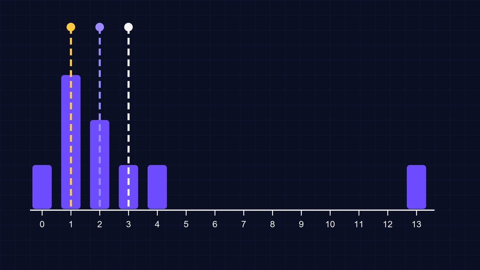
0, 1, 1, 1, 2, 2, 3, 4, 13
Questions:
- Find the mean, the median and the mode.
- Which measure best describes a “typical member” of this club? Why?
- If the member who read 13 books leaves the club, how do the three measures change?
Grab a pencil and have a go before you look at the answers.
Answers:
- Total ; mean . The data is already in order and there are 9 values; the 5th one, in the middle, is 2, so the median is 2. The value that appears most often is 1 (three times), so the mode is 1. Three measures, three different results!
- Six of the nine members read fewer than 3 books; only two read more than 3. The 13 is an outlier and has pulled the mean up. For a “typical member”, the median (2) is a better summary. If the question is “What is the most common situation?”, the mode (1) is also a meaningful answer.
- The remaining data: 0, 1, 1, 1, 2, 2, 3, 4. The total is 14 and there are 8 values, so the mean is . There is an even number of values; the two in the middle (the 4th and 5th) are 1 and 2, so the median is . The mode is still 1. The mean dropped from 3 to 1.75, while the median only went down from 2 to 1.5.
Try it with your own data: pick the first 15 words on a random page of a book and write down how many letters each word has. Work out the three measures. Then add an imaginary 30-letter word to the list and see which measure changes the most. Don’t forget to write down your prediction before you calculate!
If you’d like to strengthen these ideas with step-by-step practice, take a look at our lesson Reading data: mean, median and mode.
Summary
- The mean is the total divided by the number of values. It takes every value into account and is directly linked to the total, but it is sensitive to outliers.
- The median is the middle value of the ordered data; with an even number of values, take the mean of the two middle ones. It is robust against outliers.
- The mode is the most frequent value; there may be more than one, or none at all. It is the only measure of centre that works for categories that cannot be put in order, such as colours or cities.
- In right-skewed data, the mean often comes out above the median.
- When combining the means of groups of different sizes, use a weighted mean.
- Looking at several measures together, and at the spread as well, tells the story of the data far better than a single number.
For more on data and statistics, take a look at our Maths topics and our maths articles.
Frequently asked
5 questionsWhat is the difference between the mean, median and mode?
The mean is the total of the values divided by the number of values. The median is the middle value when the data is put in order from smallest to largest. The mode is the value that appears most often. All three summarise the centre of the data from a different angle.
How do you find the median when there is an even number of values?
First put the values in order from smallest to largest, then take the mean of the two middle values. For example, in the data 2, 3, 4, 5, 6, 40 the median is (4 + 5) ÷ 2 = 4.5.
Which measure should I use if the data has outliers?
The median usually gives a better summary, because it looks at the middle of the ordered list and is hardly affected by extreme values. The mean, by contrast, is pulled towards the outlier.
Can a set of data have more than one mode?
Yes. In the data 2, 2, 4, 6, 6, 9, both 2 and 6 appear twice, so there are two modes. If no value repeats, we usually say there is no mode.
Does the mean of two groups' means give the combined mean?
Only if the groups are the same size. Otherwise you need a weighted mean: a group of 20 with a mean of 70 and a group of 30 with a mean of 80 have a combined mean of 76, not 75.
Sources
6 sources- 1.OpenStax, Introductory Statistics 2e — 2.5 Measures of the Center of the Data (opens in a new tab)
- 2.OpenStax, Introductory Statistics 2e — 2.6 Skewness and the Mean, Median, and Mode (opens in a new tab)
- 3.Eurostat — Glossary: At-risk-of-poverty rate (opens in a new tab)
- 4.Huff, D. (1954) — How to Lie with Statistics, W. W. Norton (Chapter 2: The Well-Chosen Average)
- 5.Wikipedia — Median (opens in a new tab)
- 6.Khan Academy — Summarizing quantitative data (mean, median, mode)
- #mean
- #median
- #mode
- #outliers
- #data handling
- #statistics