What is probability? Exploring experimental and theoretical probability with dice
If the chance of rolling a 6 on a fair dice is 1/6, why don't you get exactly ten 6s in 60 rolls? We explain what probability is, how theoretical and experimental probability differ, why results move towards theory as trials grow, and share a dice activity to try at home.
In this article · 8 sections
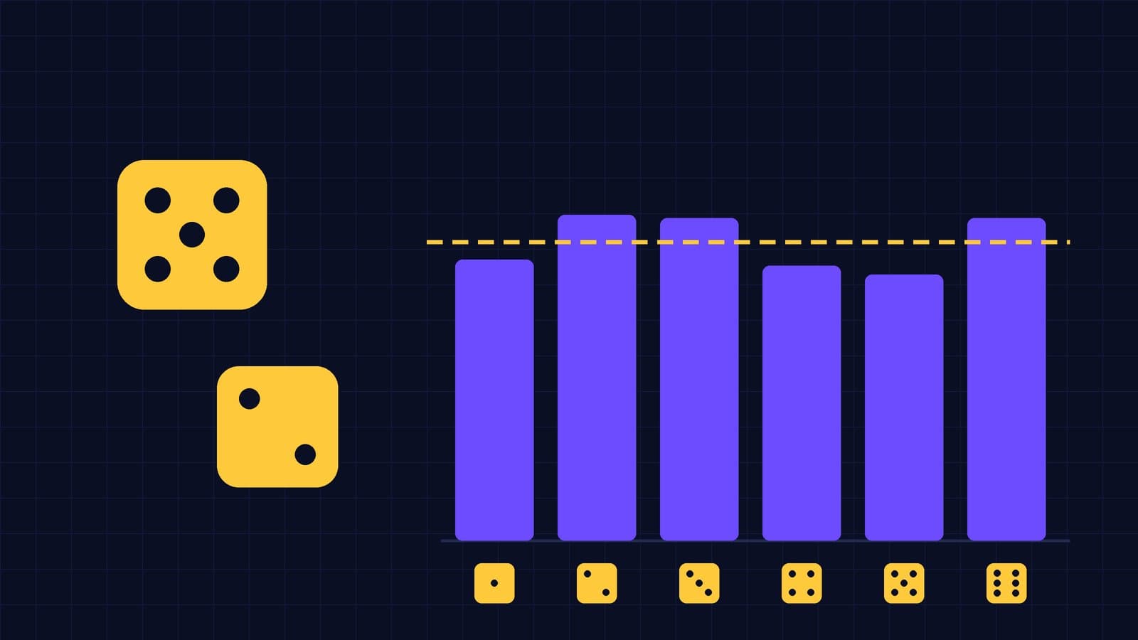
You are holding a dice. Before you roll it, someone asks: “Will it be a 6?” Nobody can say for certain. But if the question is “What’s the chance of a 6?”, most of us answer straight away: “one in six”. So where does that “one in six” come from? If you roll the dice 6 times, do you get exactly one 6? Roll it 60 times – exactly ten?
In this article we will roll a dice both on paper and for real, and meet the two faces of probability: theoretical probability and experimental probability. At the end there is a small dice activity you can try at home or in class.
What is probability?
Probability is a way of describing how likely an event is, using a number between 0 and 1. It turns up everywhere, from the chance of rain in a weather forecast to the rules of a board game.
- An event with probability 0 never happens; it is called an impossible event. Rolling a 7 on an ordinary dice is an example.
- An event with probability 1 always happens; it is called a certain event. The dice showing a number from 1 to 6 is an example.
- The values in between answer the question “how likely?”. Close to 0 means the event is rare; close to 1 means it is common.
We can write a probability as a fraction, a decimal or a percentage:
To talk about probability we need a few words. An action whose result cannot be known for certain in advance, such as rolling a dice, is called an experiment. Each possible result of the experiment is an outcome. The set of all outcomes is called the sample space, often written . For one dice:
The set of outcomes we are interested in is an event. For example, the event “rolling an even number” is . You can work through these ideas step by step, together with tree diagrams and the multiplication principle, in the Possible outcomes lesson.
Theoretical probability: working it out without rolling
The six faces of a fair dice are the same size and the dice is balanced. So there is no reason for any face to come up more easily than the others. Outcomes like these are called equally likely outcomes.
When the outcomes are equally likely, the probability of an event is given by:
Here means the number of elements in a set. This is called theoretical probability, because we find it without a single roll, just by thinking and counting.
A few examples:
- Rolling a 6:
- Rolling an even number: , so
- Rolling a prime number: the primes are 2, 3 and 5 (1 is not prime), so
- Rolling a number greater than 4: the outcomes are 5 and 6, so
The probability that an event happens and the probability that it doesn’t always add up to 1. If we write “A does not happen” as :
For example, the probability of not rolling a 6 is . If you would like to see the formula and equally likely outcomes in more detail, have a look at the Probability of simple events lesson.
A small but important note: theoretical probability is a model of an ideal dice. Real dice may not be perfectly symmetrical. Even so, a well-made dice behaves very close to this model, so the model serves us well.
Experimental probability: measuring by rolling
Now let’s put the paper down and actually roll the dice. Suppose we roll it times and the event we care about happens times. The experimental probability (relative frequency) of the event is:
The table below shows what an experiment with 60 rolls of a dice might look like. These numbers are example data; we made them up to illustrate the idea, and they are not the record of a real experiment.
| Face | Times rolled | Experimental probability | Theoretical probability |
|---|---|---|---|
| 1 | 8 | ≈ 0.133 | ≈ 0.167 |
| 2 | 12 | 0.200 | ≈ 0.167 |
| 3 | 9 | 0.150 | ≈ 0.167 |
| 4 | 11 | ≈ 0.183 | ≈ 0.167 |
| 5 | 7 | ≈ 0.117 | ≈ 0.167 |
| 6 | 13 | ≈ 0.217 | ≈ 0.167 |
| Total | 60 | 1 | 1 |
What do we notice?
- The experimental probabilities are spread around the theoretical value of , but none of them is exactly equal to it.
- In 60 rolls, the expected number for each face is . The numbers in the table range from 7 to 13. With only 60 trials, this much variation is perfectly normal.
- The experimental probabilities also add up to 1, because every roll lands on some face.
Theoretical probability stays fixed: whoever rolls the dice, it is for each face. Experimental probability, on the other hand, comes out a little differently in every experiment. If you rolled the same dice 60 times, you would get quite a different table.
We can also estimate roughly how many times an event with a known theoretical probability will happen in trials:
For example, if a dice is rolled 300 times, we expect an even number about times. The word “about” matters here: 143 or 158 would be completely ordinary too.
Experimental probability is especially valuable when we don’t know the theoretical probability. If you drop a drawing pin on a table, you cannot find the probability of it landing point up just by counting, because the two results are not equally likely. The way to find out is to drop it many times and count. You can carry on comparing experimental and theoretical probability in the Experiment and theory: experimental probability lesson.
What happens as the number of trials grows?
Is 60 rolls too few? Let’s see how the proportion of 6s changes as we roll more and more. The numbers below are also example data, made up to show what a typical experiment might look like.
| Number of rolls | Number of 6s | Expected number | Experimental probability |
|---|---|---|---|
| 6 | 2 | 1 | ≈ 0.333 |
| 60 | 13 | 10 | ≈ 0.217 |
| 600 | 94 | 100 | ≈ 0.157 |
| 6000 | 1012 | 1000 | ≈ 0.169 |
With only a few rolls, the proportion can be quite far from . As the number of rolls grows, the proportion settles into a narrower and narrower band around . This observation is known as the law of large numbers. The Swiss mathematician Jakob Bernoulli proved a mathematical form of this idea; the proof appears in his book Ars Conjectandi, published in 1713, after his death.
There is a subtle but very important detail hidden in the table. First look at the last column, the proportion: it is getting closer to the theoretical value. Now look at the difference between the number of 6s and the expected number: 1 after 6 rolls, 3 after 60, 6 after 600 and 12 after 6000. The difference is not shrinking; in this example it is actually growing. That is no accident: the typical distance between the count and the expected number grows with the square root of the number of trials, and after 6000 rolls it is about 29 (). Yet the proportion still approaches 0.167, because 12 extra 6s make up a tiny share of 6000 rolls.
So the law of large numbers does not say that the dice “corrects” its past deviations. The deviations get diluted within an ever larger number of trials. This distinction is also the key to understanding the gambler’s fallacy, which we discuss below.
This is one reason why scientists don’t settle for a single trial but repeat their measurements many times. In a small number of trials, chance can easily sway the result; across many trials, the real pattern shows through. You can explore this further, with two-dice examples, in the Law of large numbers lesson.
Two dice: why aren’t the totals equally likely?
Imagine rolling two dice together and adding the numbers on top. The total can be anything from 2 to 12, so there are 11 different totals. At first glance each total seems to have a probability of , but that is not how it works.
To see why, picture the dice in two different colours: one red, one blue. The red dice has 6 possible results and so does the blue one, so by the multiplication principle there are equally likely outcomes. “Red 1, blue 6” and “red 6, blue 1” are two different outcomes.
Now let’s count how many outcomes give each total (in each bracket, red dice first, then blue):
| Total | Outcomes | Number of outcomes | Probability |
|---|---|---|---|
| 2 | (1,1) | 1 | |
| 3 | (1,2), (2,1) | 2 | |
| 4 | (1,3), (2,2), (3,1) | 3 | |
| 5 | (1,4), (2,3), (3,2), (4,1) | 4 | |
| 6 | (1,5), (2,4), (3,3), (4,2), (5,1) | 5 | |
| 7 | (1,6), (2,5), (3,4), (4,3), (5,2), (6,1) | 6 | |
| 8 | (2,6), (3,5), (4,4), (5,3), (6,2) | 5 | |
| 9 | (3,6), (4,5), (5,4), (6,3) | 4 | |
| 10 | (4,6), (5,5), (6,4) | 3 | |
| 11 | (5,6), (6,5) | 2 | |
| 12 | (6,6) | 1 |
The numbers of outcomes add up to , which is how we can check that we haven’t skipped any. The most likely total is 7:
The least likely totals are 2 and 12, each with a probability of .
If you roll two dice many times, this “mountain” shape appears in the experimental results too: the middle totals come up often and the ones at the edges rarely. In a small experiment the mountain may look a bit lopsided; as the number of rolls grows, it approaches the shape in the table.
Try it yourself: a dice diary
You will need: one or two dice, paper and a pen; a calculator if you like.
Part 1: one dice
- Draw six columns on the paper, labelled 1 to 6.
- Roll the dice 30 times; after each roll, put a tally mark in the column for the number you got.
- Work out the experimental probability for each face: times rolled ÷ 30.
- Compare your results with the theoretical probability .
Part 2: combine your results
- Do the same experiment with a few family members or friends (30 rolls each).
- Add all the results together. With 4 people, for example, you get 120 rolls in total.
- Work out the combined proportions. Which are closer to : each person’s own proportions, or the combined ones?
Part 3: two dice
- Roll two dice 50 times and write down the total each time.
- Draw a bar chart showing how many times each total from 2 to 12 came up.
- Compare your chart with the table above. Which total came up most often? Did you get a 2 or a 12 at all?
If rolling by hand takes too long, you can repeat the same experiment thousands of times in the Coins and dice: probability simulation and watch on the chart how experimental probability approaches the theoretical value.
Questions to think about:
- If one face came up 9 times and another only 2 times in 30 rolls, does that show the dice is biased? What would you do to be more confident?
- About how many 7s would you expect in 50 rolls of two dice? ()
Educators can use this activity in class as well: each learner’s small experiment becomes part of one big experiment when the results are combined, and the law of large numbers becomes visible in the table on the board.
Things that are easily confused
“You should get one 6 in every 6 rolls”
does not mean “exactly one roll in every six will be a 6”. In 6 rolls you might get no 6s at all, or two or three. Because the rolls are independent, the probability of getting no 6 in 6 rolls is
which is roughly one in three. Probability predicts the proportion over many rolls, not individual rolls.
“If the experiment doesn’t match the theory, the dice is biased”
It can look that way at first, but deviations are normal in a small number of rolls. Getting 13 sixes instead of 10 in 60 rolls tells us almost nothing about the dice. To judge whether a dice really is unbalanced, you need far more rolls; statisticians use methods such as the chi-squared test for decisions like this.
“Two possible results means fifty-fifty”
“Either I roll a 6 or I don’t, so the probability is .” There are two kinds of result here, but they are not equally likely: “not a 6” covers five outcomes (1, 2, 3, 4, 5), while “a 6” covers just one. The counting in the formula is always done with equally likely outcomes.
“With two dice, (1, 2) and (2, 1) are the same thing”
Think about a total of 3. Even if the dice are the same colour, they are two separate objects. “First dice 1, second dice 2” and “first dice 2, second dice 1” are different outcomes. That is why the probability of a total of 3 is , not . By the same reasoning, when two coins are tossed, “one head and one tail” comes up twice as often as “two heads”.
“The dice hasn’t shown a 6 for ages, so one is due”
This way of thinking is called the gambler’s fallacy. A dice has no memory: each roll is independent of the ones before, and even if no 6 has appeared in 10 rolls, the probability of a 6 on the 11th roll is still . The law of large numbers works by dilution, not by compensation; the dice never “pays back” anything. We look at why this idea feels so convincing in our article on the birthday problem and the gambler’s fallacy.
There are situations where the past really does matter: if you draw marbles from a bag without putting them back, each draw changes what is left in the bag, so the events are dependent. You can explore the difference between independent and dependent events in the Gambler’s fallacy lesson.
Summary
- Probability describes how likely an event is with a number between 0 (impossible) and 1 (certain).
- Theoretical probability is found by counting equally likely outcomes: . On a fair dice each face has a probability of .
- Experimental probability is measured by experiment: number of times the event happens ÷ number of trials. It comes out a little differently each time.
- As the number of trials grows, experimental probability usually gets closer to theoretical probability (the law of large numbers), although the difference from the expected number need not shrink.
- Two dice have 36 equally likely outcomes; the most likely total is 7, with a probability of .
- A dice has no memory: past rolls do not change the probability of the next roll.
For more on probability and data, take a look at our Maths topics and our maths articles.
Frequently asked
5 questionsWhat is probability?
Probability describes how likely an event is with a number between 0 and 1. 0 means an impossible event and 1 a certain one. For example, the probability of rolling a 6 on a fair dice is 1/6, or about 0.167.
What is the difference between experimental and theoretical probability?
Theoretical probability is found without doing an experiment, by counting equally likely outcomes. Experimental probability is found by repeating the experiment and dividing the number of times the event happens by the number of trials, so it can come out slightly differently each time.
If you roll a dice 6 times, are you sure to get one 6?
No. The probability 1/6 describes the proportion over many rolls. The probability of getting no 6 in 6 rolls is (5/6)^6, about 0.335.
Why does experimental probability get closer to theoretical probability?
Because of the law of large numbers. As the number of trials grows, random deviations are diluted within the total and the proportion approaches the theoretical value. The dice does not make up for past deviations; they simply become a tiny share of a large total.
If a dice hasn't shown a 6 for a long time, is a 6 more likely on the next roll?
No. The rolls are independent and a dice has no memory, so the probability of a 6 is still 1/6 on every roll. Believing otherwise is known as the gambler's fallacy.
Sources
5 sources- 1.OpenStax, Introductory Statistics 2e — 3.1 Terminology (opens in a new tab)
- 2.Bernoulli, J. (1713) — Ars Conjectandi, Basel
- 3.Wikipedia — Law of large numbers (opens in a new tab)
- 4.Encyclopaedia Britannica — Law of large numbers
- 5.Khan Academy — Statistics and probability: Probability
- #probability
- #experimental probability
- #theoretical probability
- #dice
- #law of large numbers
- #relative frequency